news & articles


|
Original Aritcle by Robert Walgon on UtilityDive.com
0 Comments
From the Latham and Watkins LLP Clean Energy Law Report Blog:
On December 12, 2016, EPA published the final Formaldehyde Standards For Composite Wood Products Rule (the Rule) in the Federal Register. The compliance date for most aspects of the Rule is December 12, 2017, with a sell-through provision for wood composite products manufactured or imported prior to that date. The Rule limits formaldehyde emitted into the air from certain composite wood products, which are products made by binding strands, particles, fibers, veneers, or boards of wood together with adhesives. Domestic and foreign companies operating in the U.S. use composite wood products to manufacture a wide variety of consumer products such as furniture, flooring, cabinets, children’s toys, and more. EPA promulgated the Rule to implement the 2010 Formaldehyde Standards for Composite Wood Products Act (the Act), which Congress enacted as Title VI of the Toxic Substances Control Act (TSCA). The Act established emission standards that mirror the California Air Resource Board’s (CARB) Phase II standards for composite wood products—including hardwood plywood (HWPW), medium-density fiberwood (MDF), and particleboard (PB).[1] Similar to the California requirements, the new federal Rule regulates composite wood products from initial manufacture to final sale by (1) imposing emissions restrictions; (2) regulating product labeling, chain of custody, non-compliant product sell-through, recordkeeping and enforcement; and (3) requiring certification by EPA-approved third-party certifiers (TPC) that conduct quality assurance activities, emissions testing, inspections and auditing services. Summary of Provisions Please click here to view table. WASHINGTON — The U.S. Environmental Protection Agency has released its annual Toxics Release Inventory (TRI) National Analysis, which shows releases of toxic chemicals into the air fell 56% from 2005-2015 at industrial facilities submitting data to the TRI program.
"Today’s report shows action by EPA, state and tribal regulators and the regulated community has helped dramatically lower toxic air emissions over the past 10 years,” said Jim Jones, EPA Assistant Administrator for the Office of Chemical Safety and Pollution Prevention. “The TRI report provides citizens access to information about what toxic chemicals are being released in their neighborhoods and what companies are doing to prevent pollution.” The report shows an 8% decrease from 2014 to 2015 at facilities reporting to the program contributed to this ten-year decline. Hydrochloric acid, sulfuric acid, toluene and mercury were among chemicals with significantly lower air releases at TRI-covered facilities. Medical professionals have associated these toxic air pollutants with health effects that include damage to developing nervous systems and respiratory irritation. Combined hydrochloric acid and sulfuric acid air releases fell more than 566 million pounds, mercury more than 76,000 pounds, and toluene more than 32 million pounds at TRI-covered facilities. Coal- and oil-fired electric utilities accounted for more than 90% of nationwide reductions in air releases of hydrochloric acid, sulfuric acid and mercury from 2005 to 2015 in facilities reporting to the program. This trend is helping protect millions of families and children from these harmful pollutants. Reasons for these reductions include a shift from coal to other fuel sources, the installation of control technologies, and implementation of environmental regulations. In 2015, of the nearly 26 billion pounds of total chemical waste managed at TRI-covered industrial facilities (excluding metal mines), approximately 92% was not released into the environment due to the use of preferred waste management practices such as recycling, energy recovery, and treatment. This calculation does not include the metal mining sector, which presents only limited opportunities for pollution prevention. The TRI Pollution Prevention (P2) Search Tool has more information about how individual facilities and parent companies are managing waste and reducing pollution at the source. EPA, states, and tribes receive TRI data annually from facilities in industry sectors such as manufacturing, metal mining, electric utilities, and commercial hazardous waste management. Under the Emergency Planning and Community Right-to-Know Act (EPCRA), facilities must report their toxic chemical releases for the prior calendar year to EPA by July 1 of each year. The Pollution Prevention Act also requires facilities to submit information on pollution prevention and other waste management activities of TRI chemicals. Nearly 22,000 facilities submitted TRI data for calendar year 2015. This year’s report also includes a section highlighting the new Frank R. Lautenberg Chemical Safety for the 21st Century Act. This section focuses on the overlap between TRI chemicals and chemicals designated as Work Plan chemicals by EPA’s Office of Chemical Safety and Pollution Prevention under the Toxic Substances Control Act (TSCA). The TRI National Analysis website includes new interactive features such as an automated “flipbook” [https://www.epa.gov/trinationalanalysis/30-year-anniversary-tri-program-slideshow] depicting how the TRI Program has evolved over the past 30 years, and a new embedded dashboard that allows users to build customized visualizations of TRI data by a chemical or a sector. These features are intended to promote more user engagement and exploration of TRI data. To access the 2015 TRI National Analysis, including local data and analyses, visit www.epa.gov/trinationalanalysis Information on facility efforts to reduce toxic chemical releases is available at www.epa.gov/tri/p2. Particle Size Distributions in Method 5 Stack Samples Determined by Microscopical Methods1/13/2017 Original article: 2005:42: Vander Wood
The traditional method for determining the particle size distribution in stack emissions is gravimetric analyses of material collected on cascade impactors. But new sources have particulate loadings so low that sampling times of many hours (or days) are required to collect enough particulate for gravimetric techniques. Collection of Method 5 samples on appropriate filters followed by microscopical analysis of the collected material offers an alternative method of particle size distribution measurement, with sampling times of only minutes to hours required. Particle sizes down to 0.1 um diameter can be measured, and the particle size distribution reported in customizable cutoffs. In addition to mass fraction, number fraction of particles and estimates of particle surface area fraction can be determined for each size category. 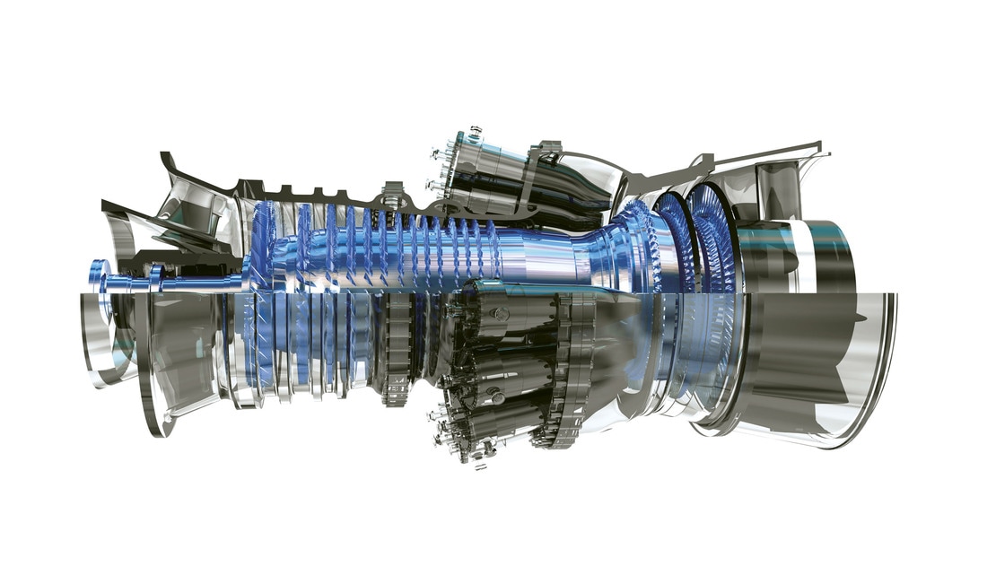 Primer video on how a gas turbine generates electricity from GE:
https://www.youtube.com/watch?v=zcWkEKNvqCA  In-field gas chromatography (GC) has long been a helpful complement to some of the more common EPA methods in the stack testing world. Although many GC approaches are very simple, some require particular care – especially when measuring reactive species such as reduced sulfur compounds. EPA Method 15 is one of the go-to approaches for reduced sulfur species (smelly gases like hydrogen sulfide, carbon disulfide and carbonyl sulfide). While the method is straightforward as written, important nuances lurk just beneath the surface. One of the more well-known factors for measuring these compounds successfully, especially at lower concentrations, is having inert materials in the sample path, from the probe, all the way to the GC column. Normally, these consist of a glass or Teflon probe, Teflon sample line, and fused silica coating on the GC inlet, valve, and sample loop (if the loop is metallic). Untreated metal fittings can lead to analyte loss, especially for hydrogen sulfide (H2S). Heating the fittings aggravates the problem. Even with all of the right materials, traces of residue from previous tests can make it difficult to obtain repeatable data. One easy, if time-consuming bit of insurance is to condition the sampling system prior to the test for several hours, by repeatedly injecting and analyzing high-level calibration gas. The good news about that is with most GC systems, this can be done using an automatic sequence, and only requires a slow stream of calibration gas. Figure 1 is an atypical, and consequently impressive example of how long a system may take to stabilize. In this example, 250ppm H2S calibration gas was injected repeatedly over 12 hours. Clearly and dramatically, the entire overnight period was needed in this case, to ensure stable measurement data. 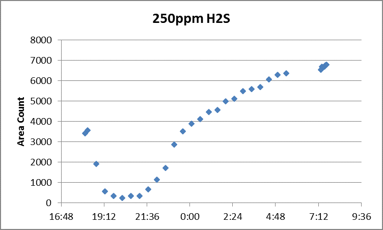 Figure 1. Overnight System Conditioning for Method 15 Happily, there is a payoff to taking such steps. Figure 2 shows the post-test calibration check for the same system – a perfectly linear calibration curve, which landed within 0.5 % of the original curve for the 55ppm low-level calibration standard. 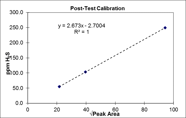 Figure 2. Post-Test Calibration Curve
So, please remember:
Original article: http://bit.ly/2iSVILY |
Archives
November 2017
|
 RSS Feed