Method 15 Ups and Downs

​In-field gas chromatography (GC) has long been a helpful complement to some of the more common EPA methods in the stack testing world.  Although many GC approaches are very simple, some require particular care – especially when measuring reactive species such as reduced sulfur compounds.  EPA Method 15 is one of the go-to approaches for reduced sulfur species (smelly gases like hydrogen sulfide, carbon disulfide and carbonyl sulfide).  While the method is straightforward as written, important nuances lurk just beneath the surface.
One of the more well-known factors for measuring these compounds successfully, especially at lower concentrations, is having inert materials in the sample path, from the probe, all the way to the GC column.  Normally, these consist of a glass or Teflon probe, Teflon sample line, and fused silica coating on the GC inlet, valve, and sample loop (if the loop is metallic).  Untreated metal fittings can lead to analyte loss, especially for hydrogen sulfide (H2S).  Heating the fittings aggravates the problem.
Even with all of the right materials, traces of residue from previous tests can make it difficult to obtain repeatable data.  One easy, if time-consuming bit of insurance is to condition the sampling system prior to the test for several hours, by repeatedly injecting and analyzing high-level calibration gas.  The good news about that is with most GC systems, this can be done using an automatic sequence, and only requires a slow stream of calibration gas.  Figure 1 is an atypical, and consequently impressive example of how long a system may take to stabilize.  In this example, 250ppm H2S calibration gas was injected repeatedly over 12 hours.  Clearly and dramatically, the entire overnight period was needed in this case, to ensure stable measurement data.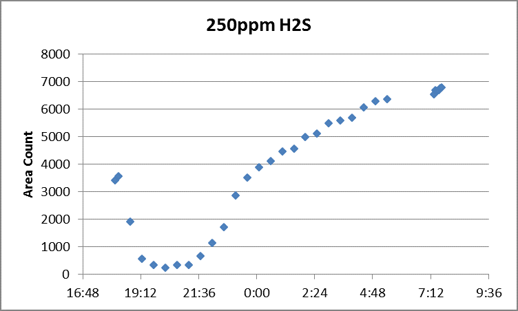

​Figure 1. Overnight System Conditioning for Method 15
Happily, there is a payoff to taking such steps.  Figure 2 shows the post-test calibration check for the same system – a perfectly linear calibration curve, which landed within 0.5 % of the original curve for the 55ppm low-level calibration standard.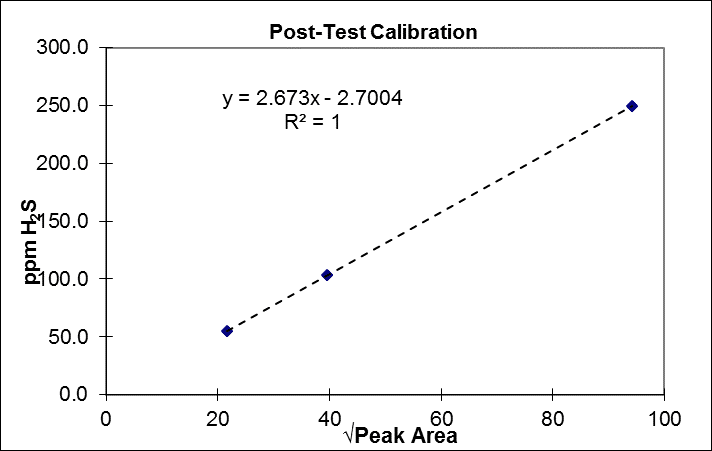

​Figure 2. Post-Test Calibration Curve
So, please remember:

• Use inert materials
• Keep the materials clean
• Condition the system before you calibrate and analyze

Original article: http://bit.ly/2iSVILY